CAPM Challenge

CAPM Challenge - Table Sliding

Find the acceleration of a ball rolling down a table using only a ball, chalk, and ruler.

Also, predict the velocity of the ball after 4 seconds.

To begin, Valentina and I set up our experiment. We raised a table up on wooden blocks to create a slant. Then, using a metronome, we marked the position of the ball at each half second as it rolled down the table.

We then measured the ball's travel from 0 seconds to 3.5 seconds. We took three trials of data and averaged all of the results. Them, we took these results and graphed the averages. 

Afterwards, we converted the centimeter measurements to meters so, when we test our data with the motion detector, it will be easier to compare. 

The equation for our line is X = 0.011t^2 + 0.0081

We know that acceleration is equal to the change in velocity/the change in time. Half the slope is equivalent to the acceleration. Since the slope of the line is equal to the velocity, we multiplied 0.011 by 2 and found the acceleration to be .022 m/s.

Then, to predict the rate of acceleration at 4 seconds, we used instantaneous velocity. 

We took our original equation X = 0.011t^2 + 0.0081 and plugged 5 in for t as well as 3.

0.011(5)^2 + 0.0081

= .2831

0.011(3)^2 + 0.0081

= .1071

Next, we subtracted the results at 5 from the results at 3. That number was then divided by two to find the instantaneous velocity of 4.

  (.2831 - .1071) / 2

= .088

We predict that the acceleration at 4 seconds will be .088 m/s

Unit 2 Summary

Unit 2 Summary - Free Bodies and Trigonometry 

In this unit, our efforts were pushed forward by force! We learned about different kind of forces, how they react upon certain objects, and how to predict the force's measurement using trigonometry.

Force: An interaction between two objects
           A push or pull (Represented as Fpush/Fpull)
         
Forces speed up, slow down, stop, and change direction but only when forces are unbalanced.
If you are pushing or pulling on an object and it does not move, the push and friction will be equal.

Normal forces are the forces perpendicular to the surface of the object in analysis. Frictional forces are the forces parallel to the surface of the object in analysis. Gravitational forces pull the object in analysis down towards the Earth.

Some forces include:  Fg - Gravity: Pull between an object and the center of the Earth (weight)
                                    Fn - Normal: Crunching/Scrunching, a perpendicular force
                                    Ff - Friction: Parallel force, sharing force between two surfaces
                                    Ft - Tension: Force along a rope/chain/etc when taut/tight
                                    Fs - Spring: Returns to it's normal state when being compressed/stretched

To express these forces, we learned how to create a force of free body diagram. They display the forces acting upon an object at any given time.
To create a force diagram, you must:
1) Sketch the system and its surroundings
2) Enclose the system within a system boundary
3) Shrink the system to a point at the center of coordinate axes with one axis parallel to the direction of motion
4) Represent all relative forces (across the system boundary) with a labeled vertex
5) Indicate which forces (if any) are equal in magnitude to other forces

Using the example of a ball being propelled into the air out of a cart, we can observe several unusual rules of force.
The ball an cart move forward at a constant velocity. When the ball is thrown into the air, there is no other force acting upon it so the ball will continue moving forward at a constant velocity.
This is proved in Newton's Third Law: An object in motion stays in motion unless acted upon by an outside force.

The motion map of the ball will remain the same no matter how it is thrown because, once the ball has left the thrower's hand, gravity is the only force acting upon it.

We also learned how to calculate net force from both the horizontal and vertical directions. For the ball, the net forces will be set up in an equation. 

fVertical = fgravity > 0N

fHorizontal = 0N

Elaborating on this information, we learned how to create Free Body Diagrams at an angle. If an object is being pulled up by a force at an angle to it's surface, than the vectors representing the angled forces are also going to be angled on the diagram.

Since the tension force is angled upwards, component forces have to be added to balance the diagram. Tension gets divided into ftx and fty.

If the object is getting pulled with a force of 38N at an angle of 55o, we could find the force of friction using trigonometry.

The cos formula will give the length of ftx, which is equal to ff. 

Cos = adjacent/hypotenuse. We are trying to find the adjacent side, since ft is the hypotenuse. 

Cos 55 = adj/38N

38(cos 55) = .8408167379

This can be rounded to a friction force of .84N

All together, in unit 2, we learned about forces and how they affect various objects. We learned how to display actions of forces with Free Body Diagrams. We learned how to calculate the net force of an object and we learned how to find the amount of force projected on an object using trigonometry. 

                                      

Weight Challenge

The Weight Challenge

Determine the weight of the unknown object hanging from two objects at unequal angels to each other

My partner Valentina and I observed the setup and found that rope A was being pulled with a tension force of 0.9N at a 37-degree angle. Rope B was being pulled with a tension force of 2.25N at a 70-degree angle.

In order to find the weight of the box, we set up a free-body diagram. 

We found that the angle between ftBy and ftAx was 90o (Degrees). Then, we subtracted 37 from 90 and found the angle between ftBy and ftA equals 53.

With this technique, we also found the angle of ftBy/ftAy and ftB to be 20o.

With this new information, we decided to use trigonometry to calculate the weights of ftAy and ftBy.

Cos = adj/hyp

Cos 20 = adj/2.25n

2.25N(cos 20) 

= 2.11N

Cos 53 = adj/0.09N

0.09N(cos 53)

= .54N

Then, we just added together 2.11 and .54 to get a total of 2.65N. Since fg is equal to ftAy+ftBy, fg will also equal 2.65N. 

Therefore, the weight of the mystery box is 2.65N.

Texting While Driving

How far will you travel in the time it takes to text "LOL" to a friend?

Our scenario involved a driver traveling 60 mph (1.6 mps).

60 Miles        1 Hour          1 Minute
________ X ________  X ________

1 Hour         60 Minutes    60 Seconds


     60 Miles                  60 Miles
_____________  =  ____________  =  1.6 mps

(60)(60) Seconds      3600 Secomds

Initial Data: We took six trials of five different people, observing how many seconds on average it                         took them to type out and send "LOL".

Total Average Texting Time : 1.17 Seconds
Velocity: 1.6 mps

To find the travel distance, we calculated the change in x.

x = vt + xo                                  
x = (1.6 mps) (1.17 s) + xo                                                * xo = The initial position of the
x = 1.87 + xo                                                                                  object at t = 0
x = 1.87 + 0

x = 1.87 miles.

So, you would travel 1.87 miles in the time that it takes to text "lol"... which is a really long time to take your eyes away from the road!
Don't text and drive!

Unit 1 Summary

Unit One Summary - So Many Graphs!

We began this unit learning about graphs. Specifically, graphing data in Excel and differentiating between the independent and dependent variables.

Independent: The one over which the experimenter has complete control - The X-Axis
Dependent: The one that responds to changes in the independent variable - The Y-Axis

These variables could then be expressed in a mathematical expression. For example, this graph as the X axis and Y axis  labeled according to the independent and dependent variables. I can create a mathematical expression by observing the slope and y-intercept.

In the expression, the x and y are replaced with the units being observed. In Example set 1, we are observing Mass in kg and Volume in m3.
So, taking the information we have, we can create an expression.


Slope = 122.99
Y - intercept = 0.0208
Mass (kg) = 122.99(m3) + 0.0208


We continued our studies by learning about graphical methods which match an equation to a curve. This is called curve fitting. When graphing a curved equation, the data can be modified to create a linear equation.

y = m(1/x) + b : As x increases, y decreases - y is inversely proportional to x

y = mx^2 + b : Y is proportional to the square of x

y^2 = mx + b : The square of y is proportional to x

Next, we moved from distance vs time graphs to motion maps. A motion map represents the position, velocity, and acceleration of an object at equally spaced times. The position of the object is represented with a dot. The arrows signify the object's velocity.

In this example, the object is traveling forward at a constant velocity.
If the object is moving quickly, the vectors (arrows) will be longer and the points will be spread further apart. The direction of the vectors changes depending on the direction of the moving object. Left-facing arrows indicate backwards movement while right-facing arrows indicate forward movement. A halt in movement or stopping point can be represented with multiple dots without an attached vector. Each dot represents the unit of time in which the object remained stationary. Finally, multiple objects can also be represented with multiple dot-vector sequences on the same motion map.

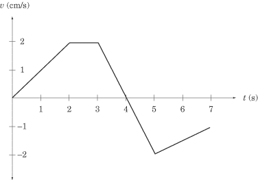
The last graph we learned about is the velocity vs time graph. This represents the velocity of the object in relation to the time it traveled.

The y - axis contains the velocity while the x - axis measures the time. The line mapping an object's travel will change depending upon the object's activity.
For example, this graph represents an object that begins traveling forward at an increasing velocity. It remains steady for two seconds before declining velocity quickly and reversing directions. It increases velocity once more before reversing back to a forward direction.


Often these graphs are compared with each other. They can express the same information by comparing different variables of data.

All of theses graphs can be represented with algebraic equations.

Velocity: - Change in Position/Time
                - Rise/Run
                - Change in x/Change in y


Constant Velocity Particle Model: x = vt + xo

                                                       X = The position of an object at any instant in time
                                                       V = The velocity of the object
                                                       T = Time
                                                      Xo = The initial position of the object at t = 0


A lot of my connections came from the labs conducted during class. For example, the Texting While Driving lab. We ran a multitude of tests to prove how dangerous texting while driving is. This genre of research produces important statistics to be considered during our everyday lives.
Also, a large majority of my math class, F2S, involves plotting on Excel and using very similar - almost identical concepts. We consider independent and dependent variables and use the equation
y = mx + b extensively. With physics, it is much easier to make a connection between math and science, bringing skills from one class into the other.